7  Control Charts for Attributes

7.1 Learning Outcomes

  • Construct and interpret p, np, c, and u charts.
  • Select the most appropriate attribute control chart based on the type of data.
  • Distinguish between proportion defective, number defective, number of nonconformities, and nonconformities per unit.

7.2 p-Chart (Proportion Nonconforming)

A p-chart monitors the proportion of defective units in a sample.
- Each item is classified as conforming or nonconforming.
- Sample size (n) can vary.

Formulae:
\[ \bar{p} = \frac{\sum d}{\sum n} \]

\[ UCL = \bar{p} + 3 \sqrt{\frac{\bar{p}(1-\bar{p})}{n}} \]

\[ LCL = \bar{p} - 3 \sqrt{\frac{\bar{p}(1-\bar{p})}{n}} \]

(If LCL < 0, set LCL = 0.)

7.2.1 Example — p-Chart

Problem:
A company inspects 10 samples of size (n = 100) electronic components each day.
The number of defective components in each sample is recorded below:

Sample Defectives (d) Sample Size (n) Proportion Defective (p)
1 8 100 0.08
2 5 100 0.05
3 12 100 0.12
4 9 100 0.09
5 7 100 0.07
6 6 100 0.06
7 10 100 0.10
8 4 100 0.04
9 11 100 0.11
10 8 100 0.08

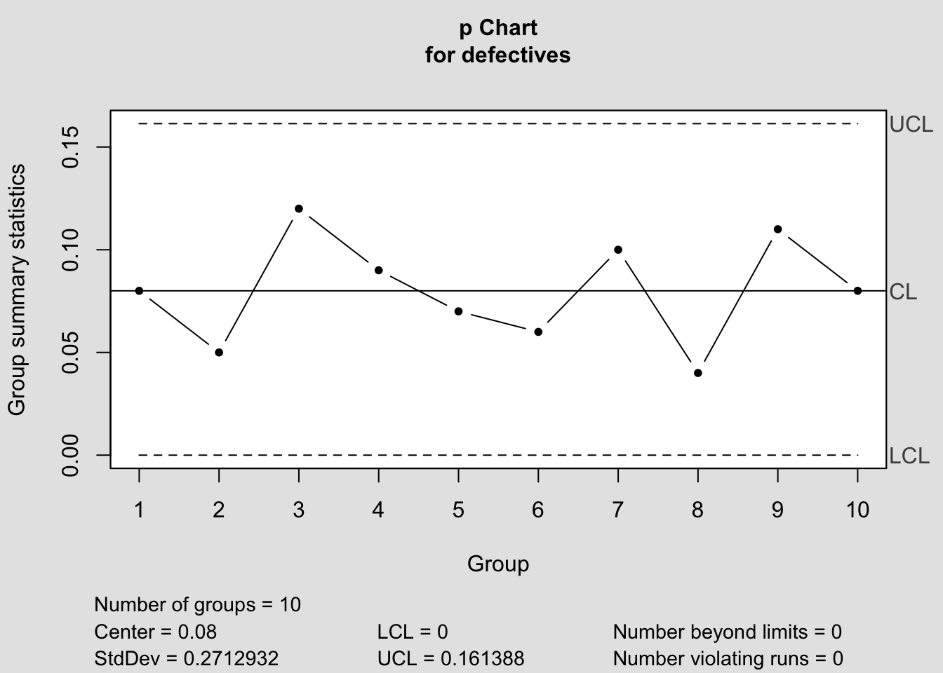
Step 1: Calculate overall proportion defective
\[ \bar{p} = \frac{\sum d}{\sum n} = \frac{80}{1000} = 0.08 \]


Step 2: Control Limits
Since (n = 100) for all samples:

\[ UCL = \bar{p} + 3 \sqrt{\frac{\bar{p}(1-\bar{p})}{n}} \] \[ = 0.08 + 3 \sqrt{\frac{0.08(0.92)}{100}} \] \[ = 0.08 + 0.0816 = 0.1616 \]

\[ LCL = \bar{p} - 3 \sqrt{\frac{\bar{p}(1-\bar{p})}{n}} \]
\[ = 0.08 - 0.0816 = -0.0016 \approx 0 \]

Thus:
- UCL = 0.162
- CL = 0.080
- LCL = 0


List of 11
 $ call      : language qcc(data = defectives, type = "p", sizes = sample_size, main = "p-Chart for Defective Components")
 $ type      : chr "p"
 $ data.name : chr "defectives"
 $ data      : num [1:10, 1] 8 5 12 9 7 6 10 4 11 8
  ..- attr(*, "dimnames")=List of 2
 $ statistics: Named num [1:10] 0.08 0.05 0.12 0.09 0.07 0.06 0.1 0.04 0.11 0.08
  ..- attr(*, "names")= chr [1:10] "1" "2" "3" "4" ...
 $ sizes     : num [1:10] 100 100 100 100 100 100 100 100 100 100
 $ center    : num 0.08
 $ std.dev   : num 0.271
 $ nsigmas   : num 3
 $ limits    : num [1:10, 1:2] 0 0 0 0 0 0 0 0 0 0 ...
  ..- attr(*, "dimnames")=List of 2
 $ violations:List of 2
 - attr(*, "class")= chr "qcc"

Step 3: Interpretation
- All sample proportions fall between 0 and 0.162.
- The process is in control.
- No evidence of special causes of variation.

The p-chart shows that all 10 samples are within control limits. Conclusion: The production process is stable with an average defect rate of 8%.

7.2.2 Exercise 1 — p-Chart

Problem:
A factory inspects samples of (n = 200) light bulbs each day for 7 days.
The number of defectives observed is given below:

Sample Defectives (d) Sample Size (n)
1 12 200
2 8 200
3 15 200
4 20 200
5 10 200
6 18 200
7 9 200

Tasks for Students:
1. Calculate the overall proportion defective \(\bar{p}\).
2. Construct a p-chart for the data.
3. Determine whether the process is in control.


7.2.3 Exercise 2 - p-Chart

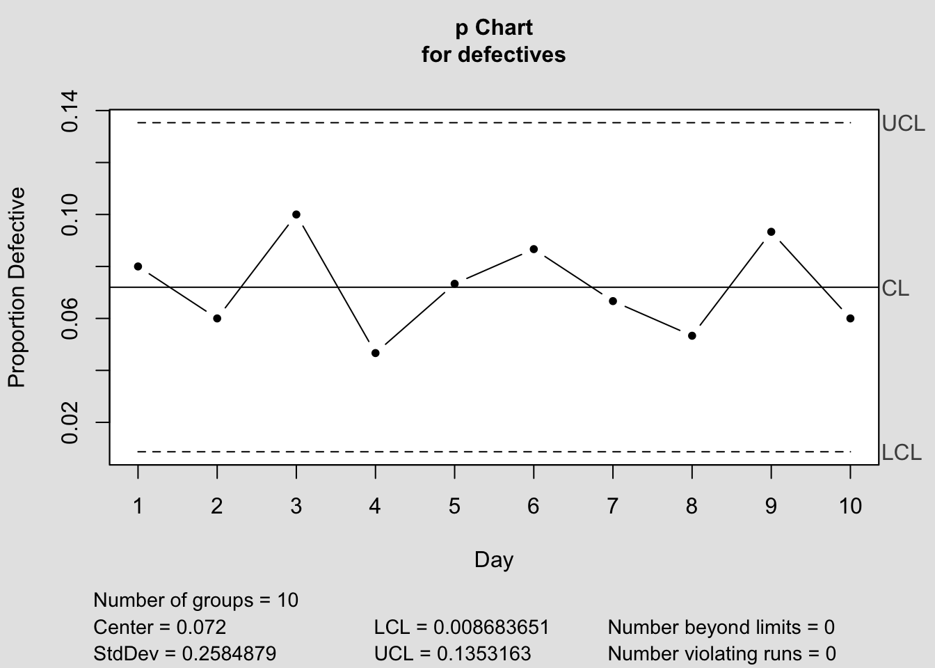
A factory inspects samples of 150 light bulbs each day for defects.
The number of defectives found over 10 consecutive days is shown below:

Day Number Defective Sample Size Proportion
1 12 150
2 9 150
3 15 150
4 7 150
5 11 150
6 13 150
7 10 150
8 8 150
9 14 150
10 9 150

Tasks for Students:
1. Construct a p-Chart for the process.
2. Calculate the center line \((\bar{p})\) and the control limits.
3. Determine whether the process is in control.


Step 1: Calculate \(\bar{p}\): \[ \bar{p} = \frac{\text{Total Defectives}}{\text{Total Inspected}} = \frac{12+9+15+7+11+13+10+8+14+9}{10 \times 150} = \frac{108}{1500} = 0.072 \]

Step 2: Control Limits: \[ UCL = \bar{p} + 3\sqrt{\frac{\bar{p}(1-\bar{p})}{n}} \quad , \quad LCL = \bar{p} - 3\sqrt{\frac{\bar{p}(1-\bar{p})}{n}} \]

\[ UCL = 0.072 + 3\sqrt{\frac{0.072 \times 0.928}{150}} \approx 0.137 \] \[ LCL = 0.072 - 3\sqrt{\frac{0.072 \times 0.928}{150}} \approx 0.007 \]

Step 3: Interpretation:
• All points fall within 0.007 – 0.137.
• No nonrandom pattern is observed.
• ✅ The process is in statistical control.

 [1] "List of 11"                                                                                                                                                   
 [2] " $ call      : language qcc(data = defectives, type = \"p\", sizes = sample_size, main = \"p-Chart for Light Bulb Defects\",      xlab = \"Day| __truncated__"
 [3] " $ type      : chr \"p\""                                                                                                                                     
 [4] " $ data.name : chr \"defectives\""                                                                                                                            
 [5] " $ data      : num [1:10, 1] 12 9 15 7 11 13 10 8 14 9"                                                                                                       
 [6] "  ..- attr(*, \"dimnames\")=List of 2"                                                                                                                        
 [7] " $ statistics: Named num [1:10] 0.08 0.06 0.1 0.0467 0.0733 ..."                                                                                              
 [8] "  ..- attr(*, \"names\")= chr [1:10] \"1\" \"2\" \"3\" \"4\" ..."                                                                                             
 [9] " $ sizes     : num [1:10] 150 150 150 150 150 150 150 150 150 150"                                                                                            
[10] " $ center    : num 0.072"                                                                                                                                     
[11] " $ std.dev   : num 0.258"                                                                                                                                     
[12] " $ nsigmas   : num 3"                                                                                                                                         
[13] " $ limits    : num [1:10, 1:2] 0.00868 0.00868 0.00868 0.00868 0.00868 ..."                                                                                   
[14] "  ..- attr(*, \"dimnames\")=List of 2"                                                                                                                        
[15] " $ violations:List of 2"                                                                                                                                      
[16] " - attr(*, \"class\")= chr \"qcc\""                                                                                                                           
7.3 np-Chart (Number Nonconforming)

An np-chart monitors the number of defective items in a sample of fixed size (n).
- Easier to interpret than p-chart when (n) is constant.

The np-Chart is a control chart used for attribute data where the number of nonconforming (defective) units in a sample is counted. Unlike the p-Chart (which monitors the proportion defective), the np-Chart directly monitors the number of defectives per sample.

7.3.1 When to Use np-Chart

  • The quality characteristic is recorded as conforming or nonconforming.
  • The sample size (n) is constant.
  • You are interested in the count of defectives, not the proportion.

Example:
- Counting the number of defective bulbs in a batch of 100 inspected bulbs daily.
- Recording the number of incomplete application forms in each group of 50.

Formulae:
\[ \bar{np} = n \cdot \bar{p} \]

\[ UCL = \bar{np} + 3 \sqrt{n \bar{p} (1-\bar{p})} \]

\[ LCL = \bar{np} - 3 \sqrt{n \bar{p} (1-\bar{p})} \]

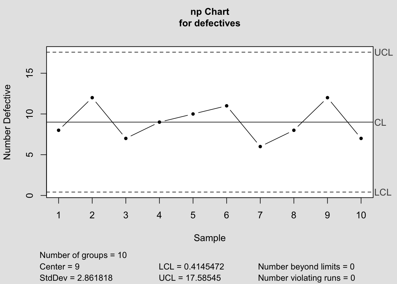
7.3.2 Example

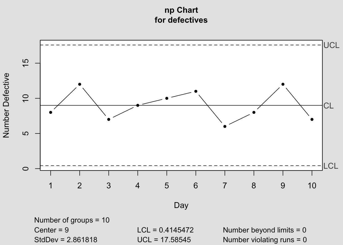
A factory inspects n = 100 bottles every day. The number of defective bottles over 10 days is recorded below:

Day Defectives
1 8
2 12
3 7
4 9
5 10
6 11
7 6
8 8
9 12
10 7

\(\bar{p} = \frac{90}{1000} = 0.09\)
\(CL = n\bar{p} = 100 \times 0.09 = 9\) \(UCL = 9 + 3\sqrt{100 \times 0.09 \times 0.91} \approx 9 + 8.64 = 17.64\)
\(LCL = 9 - 8.64 \approx 0.36 \; \Rightarrow \; 0\)

Interpretation: All points should be compared against the control limits (0 to 18). If any points fall outside or display a trend, the process may be out of control.

 [1] "List of 11"                                                                                                                                                   
 [2] " $ call      : language qcc(data = defectives, type = \"np\", sizes = sizes, main = \"np-Chart: Number of Defective Bottles\",      xlab = \"D| __truncated__"
 [3] " $ type      : chr \"np\""                                                                                                                                    
 [4] " $ data.name : chr \"defectives\""                                                                                                                            
 [5] " $ data      : num [1:10, 1] 8 12 7 9 10 11 6 8 12 7"                                                                                                         
 [6] "  ..- attr(*, \"dimnames\")=List of 2"                                                                                                                        
 [7] " $ statistics: Named num [1:10] 8 12 7 9 10 11 6 8 12 7"                                                                                                      
 [8] "  ..- attr(*, \"names\")= chr [1:10] \"1\" \"2\" \"3\" \"4\" ..."                                                                                             
 [9] " $ sizes     : num [1:10] 100 100 100 100 100 100 100 100 100 100"                                                                                            
[10] " $ center    : num 9"                                                                                                                                         
[11] " $ std.dev   : num 2.86"                                                                                                                                      
[12] " $ nsigmas   : num 3"                                                                                                                                         
[13] " $ limits    : num [1, 1:2] 0.415 17.585"                                                                                                                     
[14] "  ..- attr(*, \"dimnames\")=List of 2"                                                                                                                        
[15] " $ violations:List of 2"                                                                                                                                      
[16] " - attr(*, \"class\")= chr \"qcc\""                                                                                                                           
💡 Tip for np-Chart:
Use np-charts when the sample size is constant. If the sample size varies, use a p-chart instead.

7.3.3 Exercise 1 — np-Chart

A factory inspects 10 samples of size n = 100 bottles each.
The number of defective bottles recorded is:

Sample Number Defective
1 8
2 12
3 7
4 9
5 10
6 11
7 6
8 8
9 12
10 7

Tasks for Students:
1. Construct an np-chart for these data.
2. Interpret whether the process appears to be in control.


 [1] "List of 11"                                                                                                                                                   
 [2] " $ call      : language qcc(data = defectives, type = \"np\", sizes = sizes, main = \"np-Chart: Number of Defective Bottles\",      xlab = \"S| __truncated__"
 [3] " $ type      : chr \"np\""                                                                                                                                    
 [4] " $ data.name : chr \"defectives\""                                                                                                                            
 [5] " $ data      : num [1:10, 1] 8 12 7 9 10 11 6 8 12 7"                                                                                                         
 [6] "  ..- attr(*, \"dimnames\")=List of 2"                                                                                                                        
 [7] " $ statistics: Named num [1:10] 8 12 7 9 10 11 6 8 12 7"                                                                                                      
 [8] "  ..- attr(*, \"names\")= chr [1:10] \"1\" \"2\" \"3\" \"4\" ..."                                                                                             
 [9] " $ sizes     : num [1:10] 100 100 100 100 100 100 100 100 100 100"                                                                                            
[10] " $ center    : num 9"                                                                                                                                         
[11] " $ std.dev   : num 2.86"                                                                                                                                      
[12] " $ nsigmas   : num 3"                                                                                                                                         
[13] " $ limits    : num [1, 1:2] 0.415 17.585"                                                                                                                     
[14] "  ..- attr(*, \"dimnames\")=List of 2"                                                                                                                        
[15] " $ violations:List of 2"                                                                                                                                      
[16] " - attr(*, \"class\")= chr \"qcc\""                                                                                                                           
Answer

•   CL = average number defective = 9.
•   UCL ≈ 16, LCL ≈ 2.
•   The np-chart shows that all points fall within the control limits.
•   The process appears to be in statistical control.

7.3.4 Exercise 2 — np-Chart

A factory inspects samples of n = 80 light bulbs for defects.
The following number of defective bulbs was recorded for 10 samples:

Sample Defectives
1 6
2 9
3 4
4 7
5 8
6 5
7 10
8 6
9 9
10 7

Tasks for Students:
1. Compute the average number defective \((\bar{np})\).
2. Calculate the control limits (CL, UCL, LCL).
3. Construct the np-chart.
4. Interpret whether the process is in control.


Remember:
- \(\bar{np} = \frac{\text{Total Defectives}}{\text{Number of Samples}}\)
- \(\bar{p} = \frac{\bar{np}}{n}\) - UCL/LCL use the formula with \(3\sigma\).

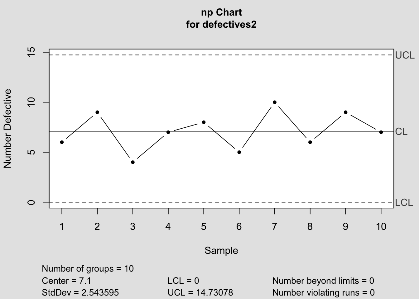
Step 1: \[ \bar{np} = \frac{71}{10} = 7.1 \]

Step 2: \[ \bar{p} = \frac{7.1}{80} = 0.08875 \]

\[ UCL = 7.1 + 3\sqrt{80 \times 0.08875 \times (1-0.08875)} \approx 14.5 \] \[ LCL = 7.1 - 3\sqrt{80 \times 0.08875 \times (1-0.08875)} \approx -0.3 ;; \Rightarrow ; 0 \]

Step 3: Plot chart above.

 [1] "List of 11"                                                                                                                                                   
 [2] " $ call      : language qcc(data = defectives2, type = \"np\", sizes = sizes2, main = \"np-Chart: Defective Light Bulbs\",      xlab = \"Sampl| __truncated__"
 [3] " $ type      : chr \"np\""                                                                                                                                    
 [4] " $ data.name : chr \"defectives2\""                                                                                                                           
 [5] " $ data      : num [1:10, 1] 6 9 4 7 8 5 10 6 9 7"                                                                                                            
 [6] "  ..- attr(*, \"dimnames\")=List of 2"                                                                                                                        
 [7] " $ statistics: Named num [1:10] 6 9 4 7 8 5 10 6 9 7"                                                                                                         
 [8] "  ..- attr(*, \"names\")= chr [1:10] \"1\" \"2\" \"3\" \"4\" ..."                                                                                             
 [9] " $ sizes     : num [1:10] 80 80 80 80 80 80 80 80 80 80"                                                                                                      
[10] " $ center    : num 7.1"                                                                                                                                       
[11] " $ std.dev   : num 2.54"                                                                                                                                      
[12] " $ nsigmas   : num 3"                                                                                                                                         
[13] " $ limits    : num [1, 1:2] 0 14.7"                                                                                                                           
[14] "  ..- attr(*, \"dimnames\")=List of 2"                                                                                                                        
[15] " $ violations:List of 2"                                                                                                                                      
[16] " - attr(*, \"class\")= chr \"qcc\""                                                                                                                           
Step 4: All points fall between 0 and 15. The process appears in control.


7.4 c-Chart (Nonconformities)

7.4.1 Introduction

A c-chart is used to monitor the number of nonconformities (defects) found in a product, process, or service, when the sample size is constant.
Unlike the p-chart or np-chart which monitor defective units, the c-chart monitors the count of defects per inspection unit (e.g., scratches, dents, holes, errors).

  • Unit of product: One physical or logical unit that can contain multiple defects.
  • Nonconformity: A specific instance of a defect, fault, or error (e.g., misspelling in a document, bubble in a paint job).
  • Each unit may have multiple defects.

7.4.2 When to Use

  • The sample (inspection area or unit) size is constant.
  • Each item can have more than one defect.
  • You want to track the total number of defects per unit over time.

Examples: - Number of typo errors per page in a report.
- Number of paint bubbles per car door.
- Number of missing stitches per garment.

Formulae:
\[ \bar{c} = \frac{\sum c_i}{k} \] \[ UCL = \bar{c} + 3 \sqrt{\bar{c}} \]

\[ LCL = \bar{c} - 3 \sqrt{\bar{c}} \]

(If LCL < 0, set LCL = 0.)

7.4.3 Construction Steps

  1. Collect defect data from (k) samples (constant size).
  2. Compute the average number of nonconformities:
    \[ \bar{c} = \frac{\text{Total Defects}}{k} \]
  3. Calculate CL, UCL, and LCL using the formulae above.
  4. Plot number of defects for each sample.
  5. Interpret the chart:
    • If points are within limits → process is in control.
    • If points fall outside limits → investigate for assignable cause.

7.4.4 Key Notes

Tip
  • p/np-chart vs. c-chart:
    • p/np-chart looks at units defective.
    • c-chart looks at number of defects, even if multiple defects occur in one unit.
Note
  • Constant area or unit is required.
    If sample size varies, use a u-chart instead.

7.4.5 Example — c-Chart for Printing Errors

A printing company monitors the number of misprints per page.
Each day, one page is selected (constant sample size = 1 page) and the number of misprints is recorded.
The data for 20 days are shown below:

Day Number of Misprints
1 3
2 5
3 4
4 2
5 6
6 3
7 7
8 5
9 2
10 4
11 3
12 8
13 6
14 4
15 5
16 3
17 4
18 2
19 5
20 6

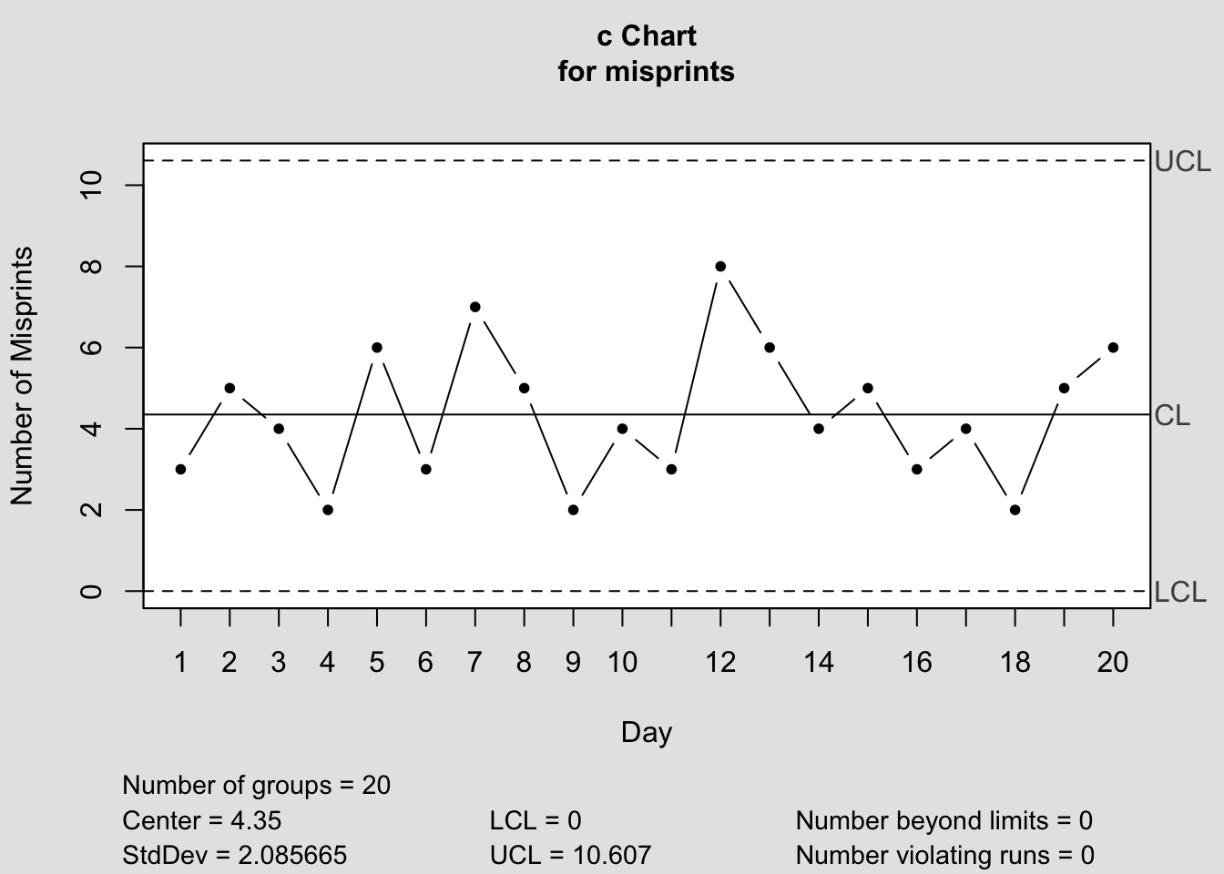
Step 1: Calculate \(\bar{c}\) \[ \bar{c} = \frac{\text{Total Misprints}}{\text{Number of Samples}} = \frac{86}{20} = 4.3 \]

Step 2: Control Limits \[ CL = \bar{c} = 4.3 \]

\[ UCL = \bar{c} + 3\sqrt{\bar{c}} = 4.3 + 3\sqrt{4.3} \approx 10.5 \]

\[ LCL = \bar{c} - 3\sqrt{\bar{c}} = 4.3 - 3\sqrt{4.3} \approx -1.9 \;\; \Rightarrow \; 0 \]

Step 3: Interpretation
- CL = 4.3
- UCL ≈ 10.5
- LCL = 0

 [1] "List of 11"                                                                                                                                                   
 [2] " $ call      : language qcc(data = misprints, type = \"c\", sizes = sizes_c, main = \"c-Chart: Misprints per Page (Daily)\",      xlab = \"Day| __truncated__"
 [3] " $ type      : chr \"c\""                                                                                                                                     
 [4] " $ data.name : chr \"misprints\""                                                                                                                             
 [5] " $ data      : num [1:20, 1] 3 5 4 2 6 3 7 5 2 4 ..."                                                                                                         
 [6] "  ..- attr(*, \"dimnames\")=List of 2"                                                                                                                        
 [7] " $ statistics: Named num [1:20] 3 5 4 2 6 3 7 5 2 4 ..."                                                                                                      
 [8] "  ..- attr(*, \"names\")= chr [1:20] \"1\" \"2\" \"3\" \"4\" ..."                                                                                             
 [9] " $ sizes     : num [1:20] 1 1 1 1 1 1 1 1 1 1 ..."                                                                                                            
[10] " $ center    : num 4.35"                                                                                                                                      
[11] " $ std.dev   : num 2.09"                                                                                                                                      
[12] " $ nsigmas   : num 3"                                                                                                                                         
[13] " $ limits    : num [1, 1:2] 0 10.6"                                                                                                                           
[14] "  ..- attr(*, \"dimnames\")=List of 2"                                                                                                                        
[15] " $ violations:List of 2"                                                                                                                                      
[16] " - attr(*, \"class\")= chr \"qcc\""                                                                                                                           
All observed points (2–8 misprints per page) fall within control limits.
Therefore, the printing process is in statistical control.

Note

Key Insight: Although some days show higher misprints (like 8), they are still below the UCL. No corrective action is needed unless points exceed the control limits or show a trend.

7.4.6 Exercise 1 — c-Chart

A hospital records the number of medication errors per day in a particular ward.
Data for 15 consecutive days are shown below:

Day Number of Errors
1 2
2 1
3 3
4 4
5 0
6 2
7 3
8 5
9 1
10 2
11 3
12 2
13 4
14 1
15 2

Tasks for Students:
1. Construct a c-chart for the data.
2. Identify the center line (CL), upper control limit (UCL), and lower control limit (LCL).
3. Interpret whether the process is in control.


 [1] "List of 11"                                                                                                                                                    
 [2] " $ call      : language qcc(data = errors, type = \"c\", sizes = sizes_c, main = \"c-Chart: Medication Errors per Day\",      xlab = \"Day\", y| __truncated__"
 [3] " $ type      : chr \"c\""                                                                                                                                      
 [4] " $ data.name : chr \"errors\""                                                                                                                                 
 [5] " $ data      : num [1:15, 1] 2 1 3 4 0 2 3 5 1 2 ..."                                                                                                          
 [6] "  ..- attr(*, \"dimnames\")=List of 2"                                                                                                                         
 [7] " $ statistics: Named num [1:15] 2 1 3 4 0 2 3 5 1 2 ..."                                                                                                       
 [8] "  ..- attr(*, \"names\")= chr [1:15] \"1\" \"2\" \"3\" \"4\" ..."                                                                                              
 [9] " $ sizes     : num [1:15] 1 1 1 1 1 1 1 1 1 1 ..."                                                                                                             
[10] " $ center    : num 2.33"                                                                                                                                       
[11] " $ std.dev   : num 1.53"                                                                                                                                       
[12] " $ nsigmas   : num 3"                                                                                                                                          
[13] " $ limits    : num [1, 1:2] 0 6.92"                                                                                                                            
[14] "  ..- attr(*, \"dimnames\")=List of 2"                                                                                                                         
[15] " $ violations:List of 2"                                                                                                                                       
[16] " - attr(*, \"class\")= chr \"qcc\""                                                                                                                            
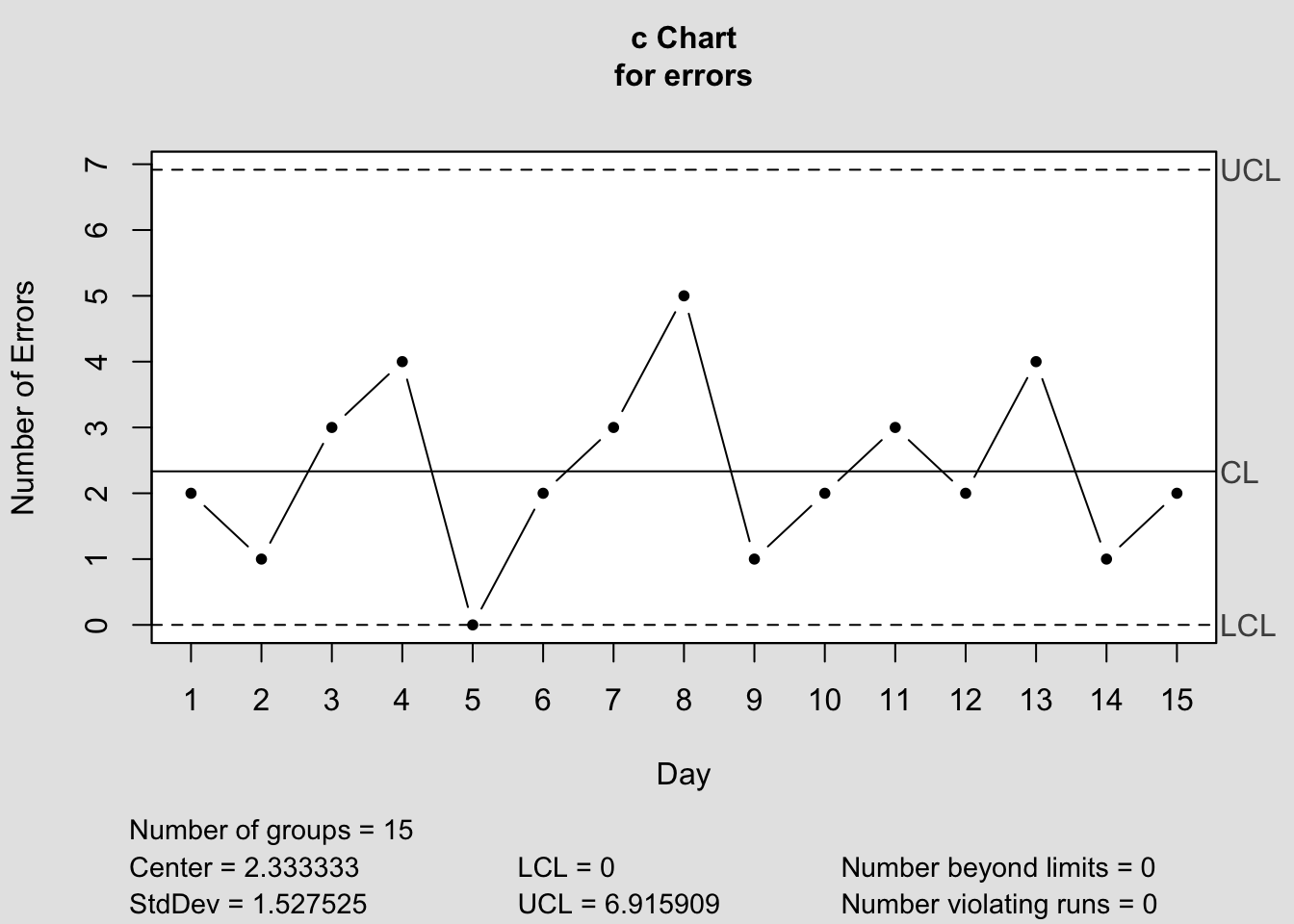
Answer:
• Average number of errors per day: \(bar{c} = 2.3\).
• UCL = \(\bar{c} + 3\sqrt{\bar{c}} \approx 6.9\).
• LCL = \(\bar{c} - 3\sqrt{\bar{c}} \approx -2.3 \Rightarrow 0\).
• All points fall within 0 and 6.9.
• ✅ The process is in statistical control.

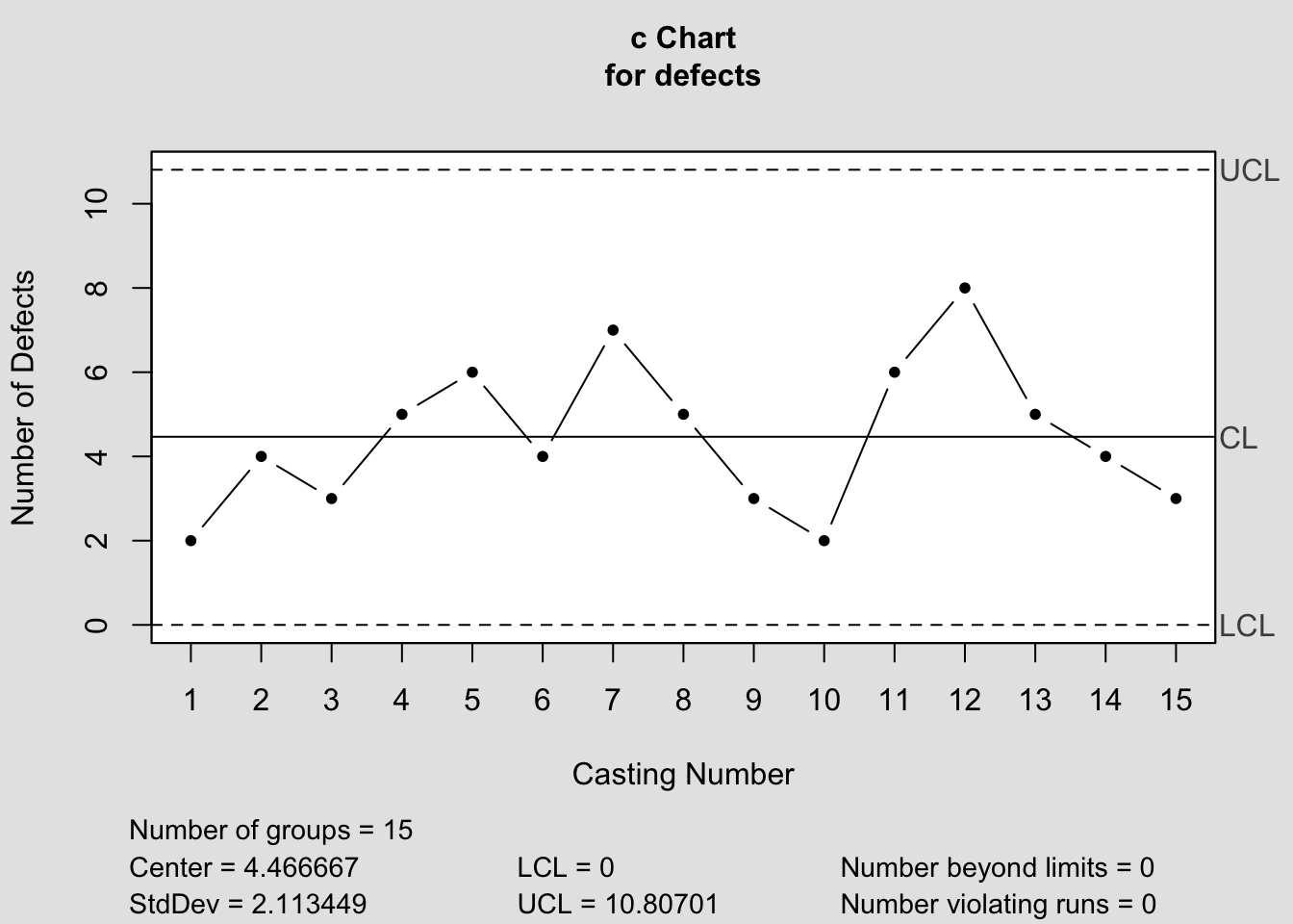
7.4.7 Exercise 2 — c-Chart (Defects in Castings)

A foundry inspects metal castings and records the number of surface defects per casting.
The results for 15 consecutive castings are shown below:

Casting No. Number of Defects
1 2
2 4
3 3
4 5
5 6
6 4
7 7
8 5
9 3
10 2
11 6
12 8
13 5
14 4
15 3

Tasks for Students:
1. Construct a c-chart for the defects.
2. Determine CL, UCL, and LCL.
3. Comment on whether the casting process is in control.


 [1] "List of 11"                                                                                                                                                   
 [2] " $ call      : language qcc(data = defects, type = \"c\", sizes = sizes_c, main = \"c-Chart: Surface Defects in Castings\",      xlab = \"Cast| __truncated__"
 [3] " $ type      : chr \"c\""                                                                                                                                     
 [4] " $ data.name : chr \"defects\""                                                                                                                               
 [5] " $ data      : num [1:15, 1] 2 4 3 5 6 4 7 5 3 2 ..."                                                                                                         
 [6] "  ..- attr(*, \"dimnames\")=List of 2"                                                                                                                        
 [7] " $ statistics: Named num [1:15] 2 4 3 5 6 4 7 5 3 2 ..."                                                                                                      
 [8] "  ..- attr(*, \"names\")= chr [1:15] \"1\" \"2\" \"3\" \"4\" ..."                                                                                             
 [9] " $ sizes     : num [1:15] 1 1 1 1 1 1 1 1 1 1 ..."                                                                                                            
[10] " $ center    : num 4.47"                                                                                                                                      
[11] " $ std.dev   : num 2.11"                                                                                                                                      
[12] " $ nsigmas   : num 3"                                                                                                                                         
[13] " $ limits    : num [1, 1:2] 0 10.8"                                                                                                                           
[14] "  ..- attr(*, \"dimnames\")=List of 2"                                                                                                                        
[15] " $ violations:List of 2"                                                                                                                                      
[16] " - attr(*, \"class\")= chr \"qcc\""                                                                                                                           
Answer: • \(\bar{c} = \frac{67}{15} \approx 4.47\).
• UCL = \(\bar{c} + 3\sqrt{\bar{c}} \approx 10.8\).
• LCL = \(\bar{c} - 3\sqrt{\bar{c}} \approx -1.9 \Rightarrow 0\).
• All points are within 0 and 10.8 → no out-of-control signals. • ✅ The process is in statistical control.


7.5 u-Chart (Nonconformities per Unit)

7.5.1 Introduction

The u-chart is an attribute control chart used when the number of nonconformities (defects) per unit is of interest, and the sample size varies.
It is an extension of the c-chart, which assumes a fixed sample size.

Applications of u-charts include:
- Monitoring the average number of defects per unit in manufacturing.
- Tracking the number of errors per invoice in accounting.
- Measuring complaints per customer in service industries.
- Monitoring accidents per man-hour in safety management.

A u-chart monitors the average number of defects per inspection unit, useful when the sample size or inspection area varies.

Formulae:
\[ u_i = \frac{c_i}{n_i} \]

\[ \bar{u} = \frac{\sum c_i}{\sum n_i} \]

\[ UCL = \bar{u} + 3 \sqrt{\frac{\bar{u}}{n_i}} \]

\[ LCL = \bar{u} - 3 \sqrt{\frac{\bar{u}}{n_i}} \]

7.5.2 Interpretation

  • The center line (CL) represents the average defects per unit.
  • The control limits vary with the sample size (n_i).
  • Points outside the limits suggest the presence of special causes of variation.
  • Patterns or trends within limits (e.g., runs) should also be investigated.

7.5.3 Example (Conceptual)

A textile company inspects rolls of fabric of different lengths.
The number of defects per roll is recorded, but since roll length varies, the sample size (in meters of fabric) differs.
A u-chart helps standardize the measure to defects per meter, allowing valid comparisons across rolls.

Advantages of u-Chart
- Adjusts naturally for variable sample sizes.
- More realistic for many real-world processes (e.g., invoices, hours worked, production runs).
- Helps avoid false signals that occur when using c-charts with varying inspection units.

Limitations
- Assumes defects occur independently and randomly.
- May be less intuitive for operators compared to simpler charts like np-chart.

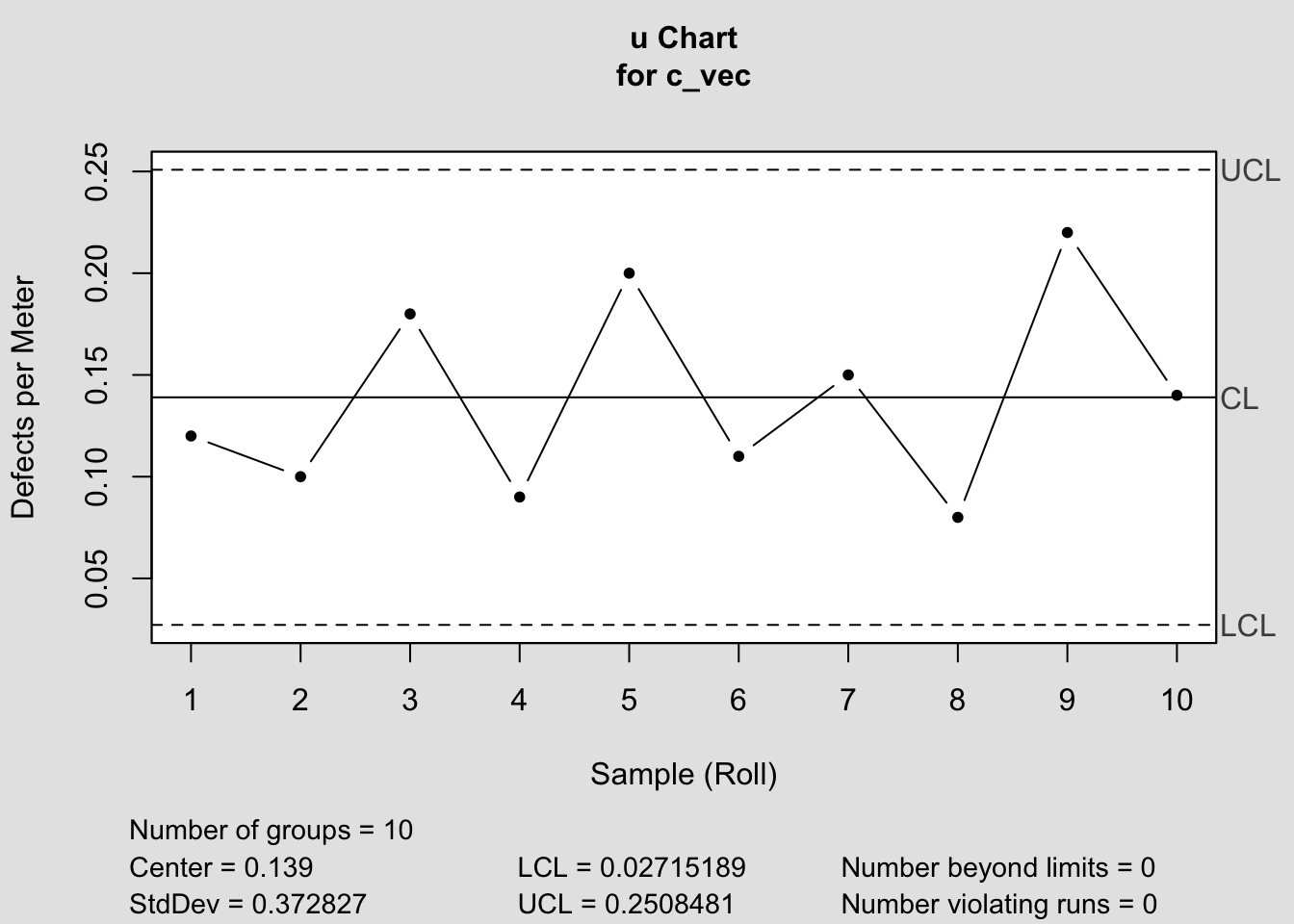
7.5.4 Exercise 1 — u-Chart

A textile mill inspects 10 fabric rolls, each of 100 meters in length.
The number of defects observed on each roll is recorded as follows:

Sample Defects (\(c_i\)) Roll Length \((n_i)\) u
1 12 100
2 10 100
3 18 100
4 9 100
5 20 100
6 11 100
7 15 100
8 8 100
9 22 100
10 14 100

Tasks: 1. Compute \(u_i = \dfrac{c_i}{n_i}\) for each sample.
2. Find the overall average \(\bar{u}\).
3. Construct a u-chart using the data.
4. Shade/plot the points on the blank control chart below.
5. Decide whether the process is in statistical control.


TipAnswer

Data: Defects per roll
\[ c = (12,\,10,\,18,\,9,\,20,\,11,\,15,\,8,\,22,\,14), \quad n_i = 100\ \text{m for all } i \]

Average nonconformities per meter \[ \bar{u}=\frac{\sum c_i}{\sum n_i}=\frac{139}{1000}=0.139 \]

Control limits (since (n_i=100) for all samples, limits are constant): \[ UCL = \bar{u} + 3\sqrt{\frac{\bar{u}}{n}} = 0.139 + 3\sqrt{\frac{0.139}{100}} \approx \mathbf{0.2508} \] \[ LCL = \bar{u} - 3\sqrt{\frac{\bar{u}}{n}} = 0.139 - 3\sqrt{\frac{0.139}{100}} \approx \mathbf{0.0272} \]

Interpretation:
\(u_i\) = \(c_i/100\) are
(0.12, 0.10, 0.18, 0.09, 0.20, 0.11, 0.15, 0.08, 0.22, 0.14);
all points lie within (0.0272) to (0.2508) → process in statistical control.

 [1] "List of 11"                                                                                                                                                  
 [2] " $ call      : language qcc(data = c_vec, type = \"u\", sizes = sizes, main = \"u-Chart: Defects per Meter (Roll length = 100 m)\",      xlab| __truncated__"
 [3] " $ type      : chr \"u\""                                                                                                                                    
 [4] " $ data.name : chr \"c_vec\""                                                                                                                                
 [5] " $ data      : num [1:10, 1] 12 10 18 9 20 11 15 8 22 14"                                                                                                    
 [6] "  ..- attr(*, \"dimnames\")=List of 2"                                                                                                                       
 [7] " $ statistics: Named num [1:10] 0.12 0.1 0.18 0.09 0.2 0.11 0.15 0.08 0.22 0.14"                                                                             
 [8] "  ..- attr(*, \"names\")= chr [1:10] \"1\" \"2\" \"3\" \"4\" ..."                                                                                            
 [9] " $ sizes     : num [1:10] 100 100 100 100 100 100 100 100 100 100"                                                                                           
[10] " $ center    : num 0.139"                                                                                                                                    
[11] " $ std.dev   : num 0.373"                                                                                                                                    
[12] " $ nsigmas   : num 3"                                                                                                                                        
[13] " $ limits    : num [1, 1:2] 0.0272 0.2508"                                                                                                                   
[14] "  ..- attr(*, \"dimnames\")=List of 2"                                                                                                                       
[15] " $ violations:List of 2"                                                                                                                                     
[16] " - attr(*, \"class\")= chr \"qcc\""                                                                                                                          
7.5.5 Exercise 2 — u-Chart

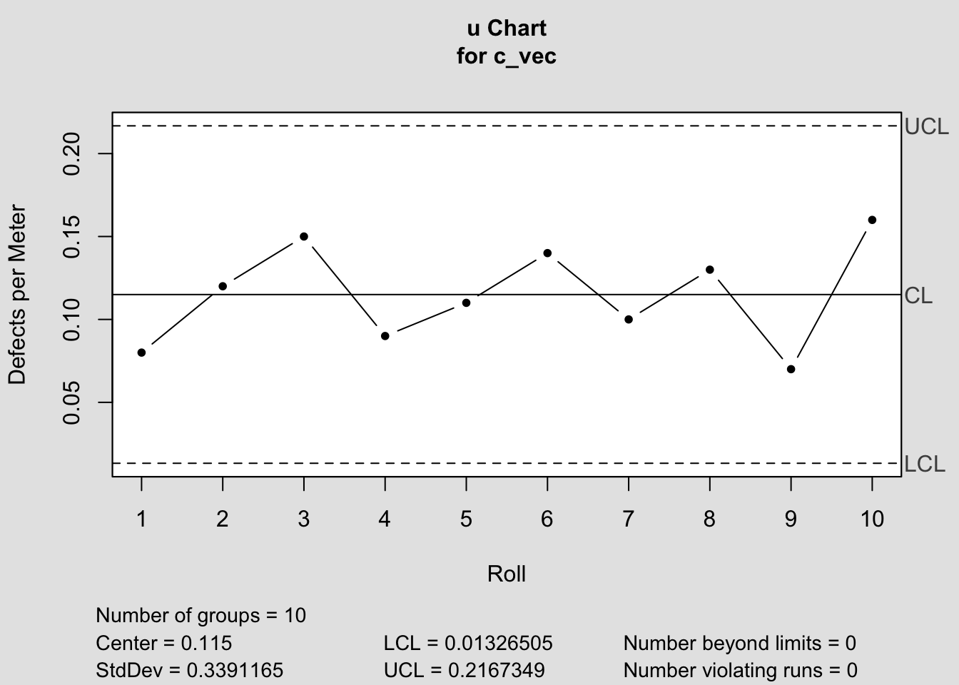
A textile factory inspects 10 rolls of fabric, each roll of equal length (100 m).
The number of defects per roll is recorded:

Roll Defects Defects per unit
1 8
2 12
3 15
4 9
5 11
6 14
7 10
8 13
9 7
10 16

Tasks for Students
1. Construct a u-chart for the data.
2. Calculate the central line, UCL, and LCL.
3. Comment whether the process is under control.

Step 1: Calculate average nonconformities per unit

\[ \bar{u} = \frac{\sum c_i}{\sum n_i} = \frac{115}{1000} = 0.115 \]

Step 2: Control limits (all rolls are 100 m each)

\[ UCL = \bar{u} + 3\sqrt{\frac{\bar{u}}{n}} = 0.115 + 3\sqrt{\frac{0.115}{100}} \approx 0.221 \]

\[ LCL = \bar{u} - 3\sqrt{\frac{\bar{u}}{n}} = 0.115 - 3\sqrt{\frac{0.115}{100}} \approx 0.009 \]

(Since LCL is positive, we keep it; if negative, set to 0.)

Step 3: Interpretation
Defect rates per roll \((u_i)\) are: 0.08, 0.12, 0.15, 0.09, 0.11, 0.14, 0.10, 0.13, 0.07, 0.16.
All points fall within 0.009 and 0.221 → process is in statistical control.

 [1] "List of 11"                                                                                                                                                    
 [2] " $ call      : language qcc(data = c_vec, type = \"u\", sizes = sizes, main = \"u-Chart: Defects per 100 m Roll\",      xlab = \"Roll\", ylab =| __truncated__"
 [3] " $ type      : chr \"u\""                                                                                                                                      
 [4] " $ data.name : chr \"c_vec\""                                                                                                                                  
 [5] " $ data      : num [1:10, 1] 8 12 15 9 11 14 10 13 7 16"                                                                                                       
 [6] "  ..- attr(*, \"dimnames\")=List of 2"                                                                                                                         
 [7] " $ statistics: Named num [1:10] 0.08 0.12 0.15 0.09 0.11 0.14 0.1 0.13 0.07 0.16"                                                                              
 [8] "  ..- attr(*, \"names\")= chr [1:10] \"1\" \"2\" \"3\" \"4\" ..."                                                                                              
 [9] " $ sizes     : num [1:10] 100 100 100 100 100 100 100 100 100 100"                                                                                             
[10] " $ center    : num 0.115"                                                                                                                                      
[11] " $ std.dev   : num 0.339"                                                                                                                                      
[12] " $ nsigmas   : num 3"                                                                                                                                          
[13] " $ limits    : num [1, 1:2] 0.0133 0.2167"                                                                                                                     
[14] "  ..- attr(*, \"dimnames\")=List of 2"                                                                                                                         
[15] " $ violations:List of 2"                                                                                                                                       
[16] " - attr(*, \"class\")= chr \"qcc\""                                                                                                                            
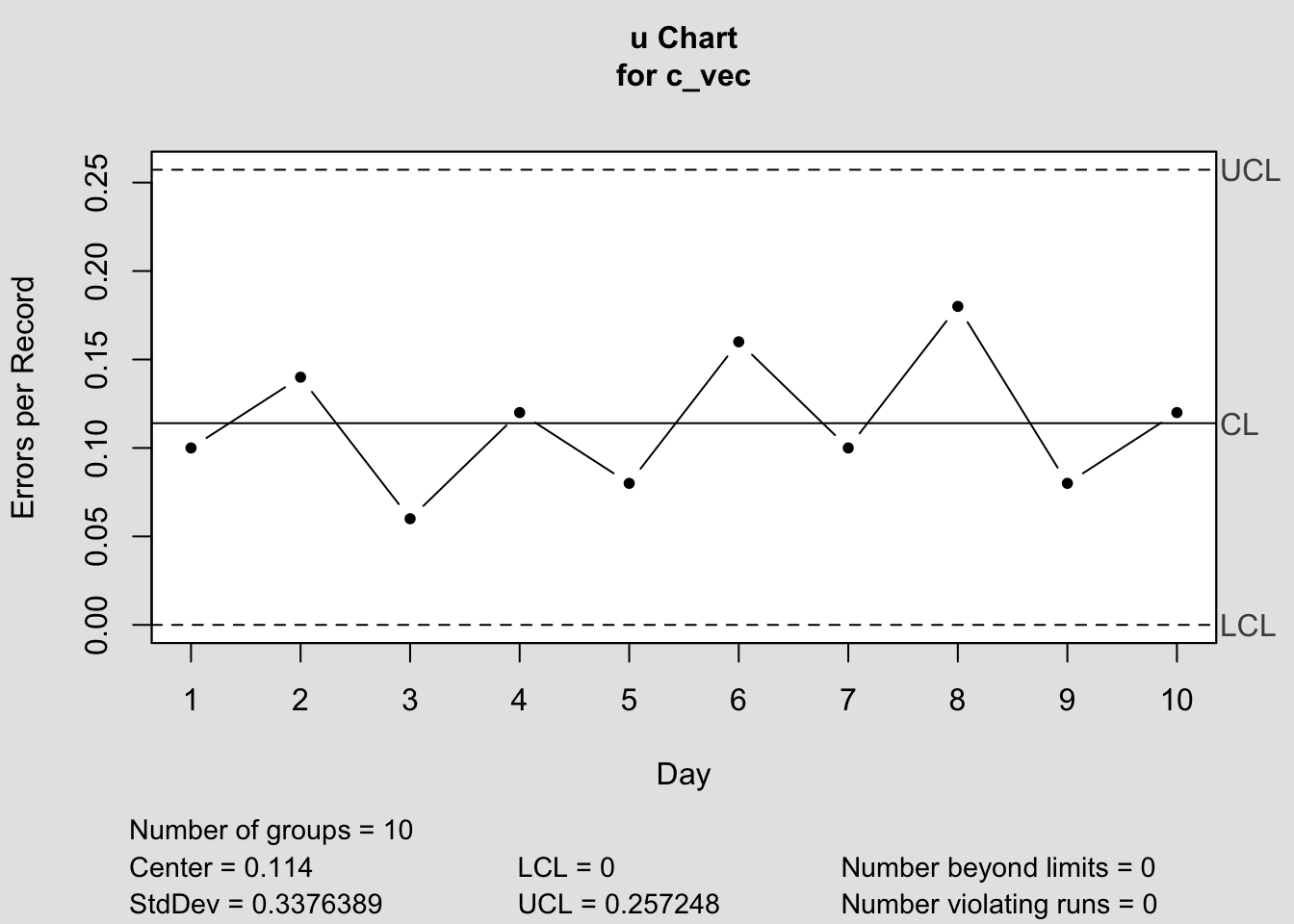
7.6 Exercise 3 — u-Chart (Service: Patient Record Errors)

A hospital’s HIM department audits batches of 50 patient records each day and counts the number of documentation errors per batch.

Day Errors (cᵢ) Records Audited (nᵢ) Error per record
1 5 50
2 7 50
3 3 50
4 6 50
5 4 50
6 8 50
7 5 50
8 9 50
9 4 50
10 6 50

Tasks for Students
1. Compute the errors per record \(u_i = c_i/n_i\) for each day.
2. Calculate the overall average \(\bar{u}\).
3. Construct a u-chart (errors per record).
4. Decide whether the process is in control.


Step 1 — \(\bar{u}\):
\[ \bar{u}=\frac{\sum c_i}{\sum n_i}=\frac{57}{500}=0.114 \]

Step 2 — Control limits (constant (n=50)):
\[ UCL=\bar{u}+3\sqrt{\frac{\bar{u}}{n}}=0.114+3\sqrt{\frac{0.114}{50}}\approx 0.257 \]
\[ LCL=\bar{u}-3\sqrt{\frac{\bar{u}}{n}}=0.114-3\sqrt{\frac{0.114}{50}}\approx -0.029\ \Rightarrow\ 0 \]

Step 3 — Interpretation:
Daily \((u_i = c_i/50 =\) (0.10, 0.14, 0.06, 0.12, 0.08, 0.16, 0.10, 0.18, 0.08, 0.12).
All points lie within [0, 0.257], with no unusual trends/runs → process in statistical control.

 [1] "List of 11"                                                                                                                                                  
 [2] " $ call      : language qcc(data = c_vec, type = \"u\", sizes = sizes, main = \"u-Chart: Documentation Errors per Record (n = 50 per day)\", | __truncated__"
 [3] " $ type      : chr \"u\""                                                                                                                                    
 [4] " $ data.name : chr \"c_vec\""                                                                                                                                
 [5] " $ data      : num [1:10, 1] 5 7 3 6 4 8 5 9 4 6"                                                                                                            
 [6] "  ..- attr(*, \"dimnames\")=List of 2"                                                                                                                       
 [7] " $ statistics: Named num [1:10] 0.1 0.14 0.06 0.12 0.08 0.16 0.1 0.18 0.08 0.12"                                                                             
 [8] "  ..- attr(*, \"names\")= chr [1:10] \"1\" \"2\" \"3\" \"4\" ..."                                                                                            
 [9] " $ sizes     : num [1:10] 50 50 50 50 50 50 50 50 50 50"                                                                                                     
[10] " $ center    : num 0.114"                                                                                                                                    
[11] " $ std.dev   : num 0.338"                                                                                                                                    
[12] " $ nsigmas   : num 3"                                                                                                                                        
[13] " $ limits    : num [1, 1:2] 0 0.257"                                                                                                                         
[14] "  ..- attr(*, \"dimnames\")=List of 2"                                                                                                                       
[15] " $ violations:List of 2"                                                                                                                                     
[16] " - attr(*, \"class\")= chr \"qcc\""                                                                                                                          
7.7 Summary

  • p-chart: proportion defective (sample size may vary).
  • np-chart: number defective (sample size fixed).
  • c-chart: number of nonconformities (fixed area/sample).
  • u-chart: nonconformities per unit (variable area/sample).

All four attribute control charts are widely used in both manufacturing and service industries, ensuring processes remain stable and sources of variation are identified quickly.